Sampling

We discuss an observation strategy for obtain a movie of M87*.

Scientifically, we are interested in the statistical properties of an M87* movie, instead of a specific movie realization. In other word, we are interested in measuring the structure function of M87*. For simplicity, we assume EHT is capable of obtaining an uniform resolution movie. We focus on estimating the time structure function for each of the pixel in such movie.

Definitions

Suppose we work with a discrete time series \(f_i = f(t_i)\). Let \(\tau_k = t_j - t_i > 0\) be a lag, the (2nd-order) discrete structure function is defined by

(7)\[\begin{align} SF(\tau_k) = \sum_{i,j}\frac{[f_i - f_j]^2}{n_k}, \end{align}\]

where \(n_k\) is the number of different \(i,j\) pairs. Note that this definition does not assume uniform time sampling \(t_i = i\Delta t\).

Nevertheless, if the function is periodic, uniform time sampling provide the same number of sampling at each lag.

Non-Periodic Function

However, this is not true for non-periodic functions. In fact, the number of sampling at each lag decreases as the lag increase. To see this, we can simply plot the histogram of the lags.

import numpy as np

def count(t):
    last  = round(t[-1])
    tau   = np.arange(last+1)
    n_tau = np.zeros(last+1)

    for ti in t:
        for tj in t:
            if tj > ti:
                tauk = tj - ti
                n_tau[round(tauk)] += 1
    return tau, n_tau

from matplotlib import pyplot as plt

N = 64
t = np.arange(N)

tau, n_tau = count(t)
plt.step(tau, n_tau, where='mid')

[<matplotlib.lines.Line2D at 0x7fc62cb65010>]

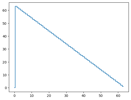
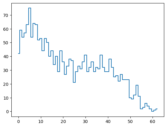
Similar trend appears for non-uniform sampling.

t = np.sort(np.random.uniform(size=N)*N)

tau, n_tau = count(t)
plt.step(tau, n_tau, where='mid')

[<matplotlib.lines.Line2D at 0x7fc62c656050>]

Golomb’s Ruler

An optimal structure function sampling would sample each \(tau_k\) the same number of time. If we want this number to be just 1, then all we need is Golomb’s Ruler. However, there are only 4 perfect rulers exist, with length up to 6. As a result, if we need to sample more than 6 different frequecies, there must be “holes” in the sampling.

t = np.array([0,1,4,13,28,33,47,54,64,70,72])

print('Order: ', len(t))
print('Length:', max(t) - min(t))

tau, n_tau = count(t)
plt.step(tau, n_tau, where='mid')

Order:  11
Length: 72

[<matplotlib.lines.Line2D at 0x7fc62cb66190>]

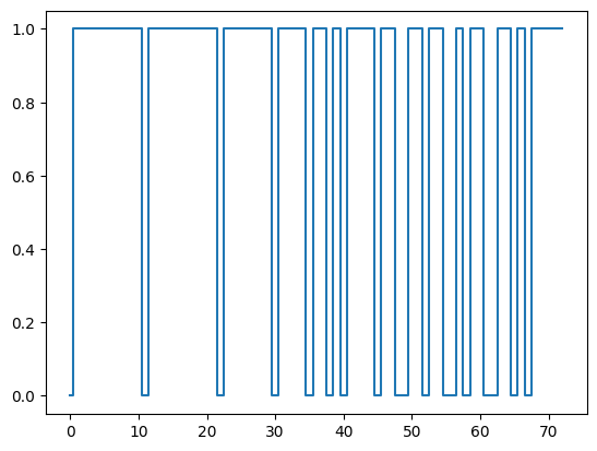
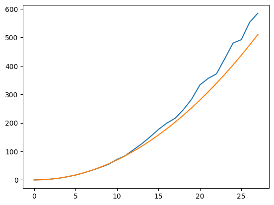
Obviously, the length of the Golomb’s Ruler grows faster than the square of its order. This suggests for a length \(N\), we need less than \(\sqrt{N}\) sampling to (almost) uniformly sampling the frequency.

orders  = np.array([1,2,3,4,5,6,7,8,9,10,11,12,13,14,15,16,17,18,19,20,21,22,23,24,25,26,27,28])
lengths = np.array([0,1,3,6,11,17,25,34,44,55,72,85,106,127,151,177,199,216,246,283,333,356,372,425,480,492,553,585])

plt.plot(orders-1, lengths)
plt.plot(orders-1, 0.7*(orders-1)**2)

[<matplotlib.lines.Line2D at 0x7fc62c4d9050>]

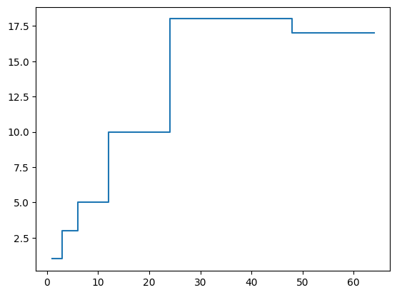
In fact, if we care about the sampling in log-frequency, the gaps do not really matter.

def countlog(t):
    last  = round(np.log2(t[-1]))
    tau   = 2**np.arange(last+1)
    n_tau = np.zeros(last+1)

    for ti in t:
        for tj in t:
            if tj > ti:
                tauk = tj - ti
                n_tau[round(np.log2(tauk))] += 1
    return tau, n_tau

tau, n_tau = countlog(t)
plt.step(tau, n_tau, where='mid')

[<matplotlib.lines.Line2D at 0x7fc62c3def90>]