Correlation

The correlation step takes signals from a pair of telescopes and computes the Fourier transform of their cross correlations. A significant property of such an operation is to remove the noise from the visibility data.

Let \(s\) be the sky signal from some radio source. When the sky signal arrives at telescopes 1 and 2, the recorded signals \(s_1\) and \(s_2\), although may have a time delay due to geometric effects, are correlated. Let \(n_1\) and \(n_2\) be noise at each of the telescopes, the cross correlation is

(1)\[\begin{align} X &= \langle (s_1 + n_1) (s_2 + n_2) \rangle \\ &= \langle s_1 s_2 \rangle + \langle s_1 n_2 \rangle + \langle s_2 n_1 \rangle + \langle n_1 n_2 \rangle. \end{align}\]

All the terms other than first term should vanishes.

By taking the Fourier transform of such a cross correlation, we obtain also the spectral information of the signal.

In this chapter, we will create synthetic very long baseline interferometry (VLBI) data and demostrate how cross-correlation can remove the noise. We will also show the XF and FX correlators are mathematically identical, although the FX correlator is computationally more efficient.

To get started, we first import the standard python packages:

import numpy as np
from math import pi, ceil
from matplotlib import pyplot as plt

Signal Generation

We consider monochromatic radio wave at unit frequency.

Using numpy, we create a time array t and then generate the recorded signals s1 and s2 at the two telescopes.

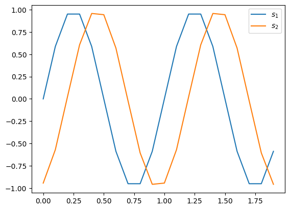
The signal at telescope 2 has a lag of \(1.2345/2\pi\) unit time compared to telescope 1.

t  = np.linspace(0, 10_000, num=100_000)
s1 = np.sin(2 * pi * t)
s2 = np.sin(2 * pi * t - 1.2345)

Plotting the two signals,

plt.plot(t[:20], s1[:20], label=r'$s_1$')
plt.plot(t[:20], s2[:20], label=r'$s_2$')
plt.legend()

<matplotlib.legend.Legend at 0x7efddcf0e450>

XF Correlator

Cross correlation is defined by:

(2)\[\begin{align} X(f, g)(\tau) = \int f^*(t) g(t + \tau) dt = \int f^*(t - \tau) g(t) dt, \end{align}\]

where \(^*\) indicates complex conjugate.

For VLBI, we only care about the discrete version of this. Hence we can replace \(g(t + \tau)\) by np.roll():

tau = 1

print(np.roll(np.arange(10), tau)) # <- this is convolution
print(np.roll(np.arange(10),-tau)) # <- this is correlation

[9 0 1 2 3 4 5 6 7 8]
[1 2 3 4 5 6 7 8 9 0]

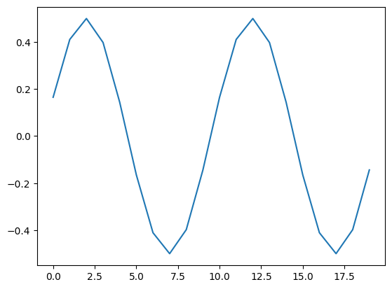
The cross correlation is simply:

X = np.array([np.mean(s1 * np.roll(s2,-tau)) for tau in range(0,100_000)])

plt.plot(X[:20])

[<matplotlib.lines.Line2D at 0x7efddc34f550>]

Applying the Fourier transform, we obtain the visibility as a function of freqnecy:

XF = np.fft.rfft(X)

plt.semilogy(abs(XF))

[<matplotlib.lines.Line2D at 0x7efddce5fc50>]

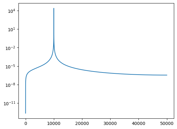
Pulling out the peak, the phase in the visibility is identical to the lag we put in:

n = np.argmax(abs(XF))
V = XF[n]

print(n)
print(abs(V))
print(np.angle(V))

10000
24188.236053877215
-1.2345033298982624

FX Correlator

Using the convolution theory, it is easy to show

(3)\[\begin{align} \widehat{X(f, g)}_k = \hat{f}_k^* \hat{g}_k. \end{align}\]

Hence, instead of first computing the cross correlation in time domain and then applying the Fourier transform, we can perform the Fourier transform first, and then compute the element-wise products in frequency domain. Correlators that use this methods are referred to as FX correlators, which can we easily implement in python:

S1 = np.fft.rfft(s1)
S2 = np.fft.rfft(s2)
FX = np.conj(S1) * S2

plt.semilogy(abs(FX))

[<matplotlib.lines.Line2D at 0x7efddc4282d0>]

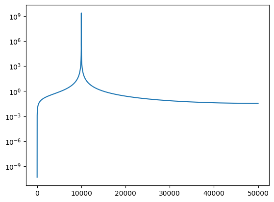
Pulling out the peak, the phase in the visibility is identical to the lag we put in, just like in the XF correlator:

n = np.argmax(abs(FX))
V = FX[n]

print(n)
print(abs(V))
print(np.angle(V))

10000
2418823605.3877215
-1.2345033298982624

Introducing Noise

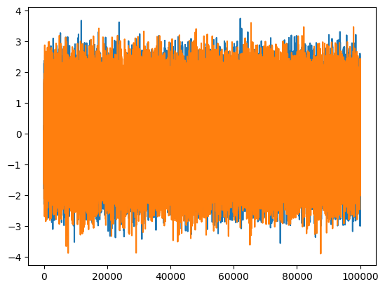
We argued at the beginning that cross correlation removes noise from the data. To demostrate this, let’s introduce noise in our simple python codes with a signal-to-noise ratio at unity.

n1 = np.random.normal(scale=np.sqrt(0.5), size=100_000)
n2 = np.random.normal(scale=np.sqrt(0.5), size=100_000)

print('SNR =', np.sum(s1*s1)/np.sum(n1*n1))
print('SNR =', np.sum(s2*s2)/np.sum(n2*n2))

plt.plot(s1 + n1)
plt.plot(s2 + n2)

SNR = 1.0007932408580766
SNR = 1.0015428778716968

[<matplotlib.lines.Line2D at 0x7efddc56ee10>]

Computing the visibility (spectrum) using the FX Correlator, we immediate see the noise floor is almost 4 orders of magnitude lower than the signal.

S1 = np.fft.rfft(s1 + n1)
S2 = np.fft.rfft(s2 + n2)
FX = np.conj(S1) * S2

plt.semilogy(abs(FX))

[<matplotlib.lines.Line2D at 0x7efddc712950>]

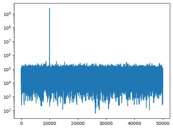
And the error in the phase is at percentage level.

n = np.argmax(abs(FX))
V = FX[n]

print(n)
print(abs(V))
print(np.angle(V))

10000
2428640294.3991523
-1.2392648071233479

Chunked Correlation

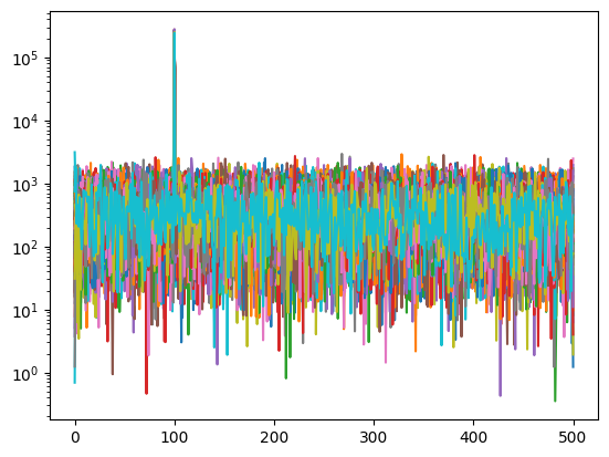
In practice, correlators do not correlate all the data in a scan all at once. In stead, they divide the signal into multiple chunks, correlate each chunk, and create a time series of visibility. Such a time series can then be averaged later to incrase the signal-to-noise ratio.

To demonstrate such process, let’s choose a chunk size of 1000, perform FX correlation over each chunk, and plot all of the resulting visibilities as function of frequency.

nc = 1000
Nc = int(ceil(len(s1) / nc) * nc)
S1 = np.fft.rfft(np.pad(s1+n1, (0, Nc-len(s1))).reshape(Nc//nc, nc))
S2 = np.fft.rfft(np.pad(s2+n2, (0, Nc-len(s2))).reshape(Nc//nc, nc))
FX = np.conj(S1) * S2

for fx in FX:
    plt.semilogy(abs(fx))

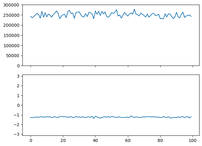
We may also look at only the “reference frequency” and plot the amplitude and phase as function of time:

n = np.argmax(abs(FX[0]))
V = FX[:,n]

print(n)

fig, (ax0, ax1) = plt.subplots(2,1, sharex=True)
fig.tight_layout()

ax0.plot(abs(V))
ax0.set_ylim(0, 300_000)

ax1.plot(np.angle(V))
ax1.set_ylim(-pi, pi)

100

(-3.141592653589793, 3.141592653589793)

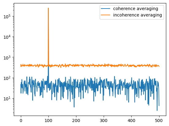
We can also perform both the coherence and incoherence averaging of the data:

plt.semilogy(abs(np.mean(FX, axis=0)), label='coherence averaging')
plt.semilogy(np.mean(abs(FX), axis=0), label='incoherence averaging')
plt.legend()

<matplotlib.legend.Legend at 0x7efddc1da490>